Play Bach: let a neural network play for you. Part 2

I do not know how to play music. But I can still play with music.

This is part of a series of articles, which will explore many aspects of this project, including static MIDI file generation, real time streaming, Tensorflow/Keras sequential and functional models, LSTM, over and under fitting, attention mechanism, embedding layers, multi-head models, probability distribution, conversion to TensorflowLite, use of TPU/hardware accelerator, running application on multiple platforms (Raspberry PI, edge devices) ….

See Part 1. Part3.

The entire code is available on github

Let’s go thru the process of preparing data and training our first neural network.

Trained on Goldberg Variations. Played with Trumpet

The Data.

The first step is to get some MIDI files of your favorite composer. Then you can use the Music21 python library to extract a sequence of notes from those MIDI files.

For this tutorial, I selected the Suites for Solo Cello , BWV 1007 to 1012 (I love Pablo Casals)

This corpus has a total of 32487 notes/chords/rests (example of the first 10 elements: [‘G2’, ‘R’, ‘R’, ‘D3’, ‘B3’, ‘A3’, ‘B3’, ‘D3’, ‘B3’, ‘D3’]) and 129 unique notes/chord (example of first 5: [‘A2’, ‘A2.F#3’, ‘A2.F3’, ‘A3’, ‘A3.B3’])

As you remember ( ref. Part 1 ), a neural network accepts only numbers for inputs. A simple method to convert notes/chords into integers is to create a dictionary, such as (‘A2’, 0), (‘A2.F#3’, 1), (‘A2.F3’, 2), (‘A3’, 3), (‘A3.B3’, 4), etc. In that sequence, the note A2 is represented by integer 0, the chord ‘A2.F’ by integer 1 and so on…

The next step is to convert the corpus into actual training data. A training sample is a sequence of (n+1) notes. I use n=40 and will explain why later. From my corpus of 32487 elements, I therefore obtain a list of 32447 training samples. Each sample is a list of 40 integers (the 40 notes) followed by one more integer (the 41th note).

Lists are python objects, but neural networks want to be fed with tensors. Think of a tensor as a multidimensional matrix of numbers. The process of converting lists into tensors is called vectorization. Once completed, the tensors are ready to be fed into the network to train it.

As a side note: Neural networks allow for a LOT of parallelism in tensor processing and one computing architecture is optimized for tensor: GPU, aka Graphic Processing Unit, aka your good old gamer graphic card. Don’t even thing of training any decent network if you do not have a GPU. Training on a general purpose CPU, even the fastest one, will be unbearable

Our first Model.

The word ‘deep’ in Deep Learning means that a neural network is a stack of layers, and there are many of them (it’s a deep stack).

The picture below depicts the stacking of our first model.

Our neural network consists of four types of layer:

• The input layer: At the top of the stack, this layer ‘receives’ the training data (tensors). The [None, 40, 129] means the network expects input tensors as a sequence of 40 numbers, each number being a value between 1 and 129. This is how we prepared our training data, so all is good. The None means the network does not care how many samples will be available (in our case 32447)
• The output layer (called softmax) is the bottom layer. The (None, 129) means that, given an input tensor (a sequence of 40) the network will predict the 41th, and this can be any value between 1 and 129 (i.e. any note/chord the network knows about).
• The processing layers: In this case they are LSTM, aka Long Short Term Memory (wouldn’t it be good if such layer were also available to us, human ?). There are two LSTM layers in our stack. Suffice to says that LSTMs are specialized in learning from sequences.
• Some white magic in the form of Normalization, ReLU, Dropout. Those layers essentially makes sure the network does not go wild during training.

The number of LSTM layers (2 in our case) and the size of them (300) are called hyperparameters. The setting of these hyperparameters is yours and there are no fixed rules. It is your skill, your intuition. It’s trial and error process. Just find a configuration that gives good result and does not take ages to train.

With this configuration, our neural network contains 1,278,429 internal variables. This is more than one million and still, it is a very small number in deep learning land. Those variables are initialized at random and the training magic is to tune them so that, at the end, they collectively recognize a cat from a dog, or in our case, predict the 41th note, given the previous 40 ones.

Training the Model with the Data.

The training process is a loop:

• grab a training sample (40 integers, representing 40 notes), and convert it to a tensor
• input this tensor into the model (i.e. into the input layer)
• the neural network will then perform a LOT of tensor operations, which involves the internal variables; at the end the network will generate a prediction for what is the 41th note (amongst the 129 notes/chords it knows about).
• the training process will then look at whether the network is right, i.e. is the prediction the actual 41th note. Think about this step as computing an ‘error’ between the network prediction and the ‘ground truth’ , which we know, as during training, we know the real value of the 41th note.
• if not right, an algorithm tunes the internal variables, so that next time the same tensor is presented to the network, the network’s prediction will be closest to the truth, i.e. the error will be lower (formally lower, there is a theorem there). Off course, at the start of training, there is zero possibility the network is right (remember the computing is based on internal variables initialized at random).
• repeat Ad Nauseam

There is nothing more to it.

In reality, this is done a bit differently, but the principle stays the same:

• the network is typically fed with many training sample at once. This is called a batch (eg 64 samples). The error computing and the internal variables tuning algorithm runs after each batch.
• when all the available training samples have been fed, then … start again. One such cycle is called an epoch.
• Training stops when the error is ‘small enough’ or does not significantly decreases after each epoch (no need to waste computing resources).
• You (the human) actually go and have a cup of coffee while your GPU turns electricity into heat.

At the end, the network will have the lowest possible error that can be achieved with the available training samples, together with the selection of network architecture and of hyperparameters. And the value of the 1.2 millions variables is the trained network.

The catch, and how to watch your model.

The error mathematically decreases after each batch/epoch ? Looks too good to be true. And yes there is a catch. The network only gets better when processing the training samples. There is no guarantee the network will have good performance on other inputs (see part 1 about generalization).

The objective therefore is to make sure the network will perform well (low errors, accurate prediction) on inputs outside the training set, i.e. ‘unseen inputs’.

To check whether this is actually happening, the available training data is split in 3 sets:

• the ‘training set’: the bulk of the data, and used for actual training. This set will be ‘seen’ by the network batch after batch, epoch after epoch.
• the ‘validation set’: not used for the internal variable tuning algorithm (I spill the bean, this algorithm is called stochastic gradient descent and use partial derivatives algebra), but rather used to compute the error/accuracy after each epoch. The evolution of error on the validation set is therefore a good indication whether the training is going well.
• the ‘test set’: never used during training, but to compute the performance of a fully trained model. The test set is used to, in a way, ‘surprise’ the model, because there is no way on earth the model had any chance to ‘adapt’ to this data during training. It is the best proxy for model performance once in operation.

Look at the graphs below to see training happening (loss in the fancy name for ‘error’), specially the accuracy plot (accuracy is a measure of the percentage of time the network predicted right).

The graph’s vertical axis is accuracy for both the training set and the validation set; the graph’s horizontal axis is epoch. As expected, accuracy on the training set (automatically) increases. What is to be monitored is accuracy on the validation set. In our case it increases and plateau to ~60% accuracy after ~50 epochs. 60% is the maximum accuracy of this model, and it is not worth to compute more epoch.

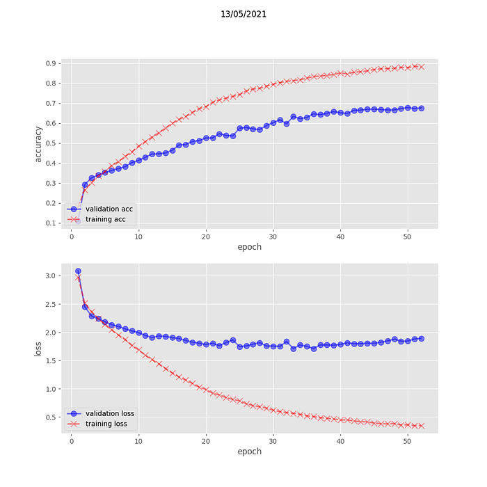
Note that 60% accuracy means the network did learned something. There are 129 possible outputs, and if the network was guessing at random, it would be right 1/129 i.e. 0,7% of the time, not 60%.

If 60% accuracy is not good enough, then go back to your model architecture, to your choice of hyper parameters, get more, better training data …. and try again.

In the next section, we shall look at what could go wrong during training, and how to use the trained model to generate actual music.

Stay tuned !!!!

— — — — — Do not cross this line if you are not interested in details —- — — —

This is the actual Tensorflow code to define our model.

The line 1 to 16 describes the various layers in our deep learning model.

Then, in line 18 to 22, some specific algorithms are selected to be used in training:

• how to mathematically compute the error
• what method to use to tune the internal variables (in our case ‘adam’, this is the name of an algorithm, there are many others)
• what metric should the training algorithm computes (it always computes loss, and we also want accuracy)

The ‘compile’ instruction creates the model. Is is not trained yet. You shall see this part in next part

So , was crossing the line worthwhile ?